Customised extensions with halomod

In this tutorial, we use the existing infrastructure of halomod and plug in a new type of tracer, namely HI using the model from arxiv:2010.07985. This model requires three additions: a new density profile for HI; a new concentration-mass relation for HI; and finally a new HI HOD.

halomod is extremely flexible. You can add custom models for any “component” (eg. mass functions, density profiles, bias functions, mass definitions,…). However, most likely you’ll need to add something to build a new type of tracer, which is the case here.

Let’s import a few basic things first:

%matplotlib inline
import hmf
import matplotlib.pyplot as plt
import numpy as np

import halomod
from halomod import TracerHaloModel

print(f"Using halomod v{halomod.__version__} and hmf v{hmf.__version__}")

Using halomod v2.0.2.dev51+geee0902 and hmf v3.5.0

Creating a new density profile

The HI density profile used here is:

\[\rho_{\rm HI} = \rho_s \bigg(\frac{r_s}{r}\bigg)^b {\rm exp}\bigg[-a \frac{r}{r_s}\bigg]\]

Notice that all the infrastructure has been set up by the Profile or ProfileInf class, depending on if you truncate the halos or not. And all you need to modify is the _f function, and optionally its integration _h and its Fourier transform _p (see documentation for `profiles.py <https://halomod.readthedocs.io/en/docs/_autosummary/halomod.profiles.html#module-halomod.profiles>`__). Note that these latter two are useful to speed up calculations, but are in principle optional and will be calculated numerically.

The _f function is:

\[f(x) = \frac{1}{x^b}{\rm exp}\big[-ax\big]\]

The integration in this case is:

\[h = \Gamma(3-b)\times a^{b-3}\]

where \(\Gamma\) is the Gamma function

The Fourier Transformed profile is:

\[p(K)= {\rm tan}^{-1}(K/a)/K,\,b=2\]

\[\begin{split}\begin{split} p(K)=&\frac{-1}{1+(K/a)^2}\Bigg(\bigg(1+K^2/a^2\bigg)^{b/2}\times\\ &\Gamma(2-b)\sin\bigg[(b-2){\rm arctan}\big[K/a\big]\bigg]\Bigg),\,b\ne2 \end{split}\end{split}\]

from scipy.special import gamma

from halomod.profiles import ProfileInf

class PowerLawWithExpCut(ProfileInf):
    """
    A simple power law with exponential cut-off, assuming f(x)=1/x**b * exp[-ax].
    """

    _defaults = {"a": 0.049, "b": 2.248}

    def _f(self, x):
        return 1.0 / (x ** self.params["b"]) * np.exp(-self.params["a"] * x)

    def _h(self, c=None):
        return gamma(3 - self.params["b"]) * self.params["a"] ** (self.params["b"] - 3)

    def _p(self, K, c=None):
        b = self.params["b"]
        a = self.params["a"]
        if b == 2:
            return np.arctan(K / a) / K
        else:
            return (
                -1
                / K
                * ((a**2 + K**2) ** (b / 2 - 1) * gamma(2 - b) * np.sin((b - 2) * np.arctan(K / a)))
            )

At bare minimum, you must specify _f which is just the density profile itself, and all the integration and Fourier transformation will be done numerically. However, that is very inefficient so you should always find analytical expression and specify if you can.

Now let’s plug it into a halo model:

hm = TracerHaloModel(tracer_profile_model=PowerLawWithExpCut, transfer_model="EH")

Note that as of v2 of halomod, defining a new model for any particular component will automatically add it to a registry of ‘plugins’, and you may then construct the overall model using a string reference to the model (i.e. we could have passed tracer_profile_model="PowerLawWithExpCut").

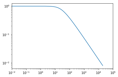
And see the profile for a halo of mass \(10^{10} M_\odot h^{-1}\) in Fourier space:

plt.plot(hm.k, hm.tracer_profile_ukm[:, 1000])
plt.xscale("log")
plt.yscale("log")
plt.xlim((1e-2, 1e5));
# plt.ylim((1e-1,1))

And we’ve set up our profile model.

This profile model has 2 additional model parameters. You can always update these parameters using:

hm.tracer_profile_params = {"a": 0.049, "b": 2.248}

Creating a new concentration-mass relation

The concentration-mass relation we use here follows the one from Maccio et al.(2007):

\[c_{\rm HI}(M,z) = c_0 \Big(\frac{M}{10^{11}{\rm M_\odot h^{-1}}}\Big)^{-0.109}\frac{4}{(1+z)^\gamma}\]

Again, because halomod already has a generic CMRelation class in place, all you really need is to specify a cm function for the equation above:

from hmf.halos.mass_definitions import SOMean

from halomod.concentration import CMRelation

class Maccio07(CMRelation):
    """
    HI concentration-mass relation based on Maccio et al.(2007).
    Default value taken from 1611.06235.
    """

    _defaults = {"c_0": 28.65, "gamma": 1.45}
    native_mdefs = (SOMean(),)

    def cm(self, m, z):
        return (
            self.params["c_0"] * (m * 10 ** (-11)) ** (-0.109) * 4 / (1 + z) ** self.params["gamma"]
        )

Note that for the concentration-mass relation that you put in, you need to specify the mass definition that this relation is defined in. In this case, it is defined in Spherical-Overdensity method, which is the default.

And set this to be the model for the tracer concentration-mass relation:

hm.tracer_concentration_model = Maccio07

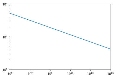
And check the concentration-mass relation at z=0:

plt.plot(hm.m, hm.tracer_concentration.cm(hm.m, 0))
plt.xscale("log")
plt.xlim(1e5, 1e15)
plt.ylim((1e1, 1e3))
plt.yscale("log");

Notice that this model has two additional parameters, which can be updated using:

hm.tracer_concentration_params = {"c_0": 28.65, "gamma": 1.45}

See the documentation for `concentration.py <https://halomod.readthedocs.io/en/docs/_autosummary/halomod.concentration.html>`__ for more.

Creating a new HOD

The HI HOD we use here is:

\[\begin{split}\begin{split} \langle M_{\rm HI}^{\rm cen}(M_h) \rangle = M_h& \Bigg[a_1^{\rm cen}\bigg(\frac{M_h}{10^{10} M_\odot}\bigg)^{\beta_{\rm cen}} {\rm exp}\Big[{-\bigg(\frac{M_h}{M^{\rm cen}_{\rm break}}\bigg)^{\alpha_{\rm cen}}}\Big] \\&+a_2^{\rm cen}\Bigg] {\rm exp}\Big[{-\bigg(\frac{M_{\rm min}^{\rm cen}}{M_h}\bigg)^{0.5}}\Big] \end{split}\end{split}\]

\[\begin{split} \langle M_{\rm HI}^{\rm sat}(M_h) \rangle = M_0^{\rm sat}\bigg( \frac{M_h}{M^{\rm sat}_{\rm min}}\bigg)^{\beta_{\rm sat}} {\rm exp}\Big[{-\bigg(\frac{M^{\rm sat}_{\rm min}}{M_h}\bigg)^{\alpha_{\rm sat}}}\Big] \end{split}\]

For the HOD, it’s a bit more complicated. First, one needs to decide what type of tracer it is. The most generic class to use is HOD, however, you may prefer HODBulk where the tracer is considered to be continuously distributed ; or HODPoisson, which assumes Poisson distributed discrete satellite components, which is commonly used for galaxies.

Second, if your model has a minimum halo mass to host any tracer as a sharp cut-off (or not), you should specify in your model definition

sharp_cut = True # or False

If your model has a seperation of central and satellite components, you need to specify if the satellite occupation is inherently dependent on the existence of central galaxies:

central_condition_inherent = False # or True

If False, the actual satellite component will be your satellite occupation times occupation for central galaxies.

See the documentation for `hod.py <https://halomod.readthedocs.io/en/docs/_autosummary/halomod.hod.html>`__, or the reference paper for more.

Finally, you need to specify how to convert units between your HOD and the resulting power spectrum. For example, for HI the HOD is written in mass units, whereas the power spectrum is in temperature units. This is done by specifying a unit_conversion method.

Additionally, sometimes your HOD contains methods that need to be calculated, such as virial velocity of the halos, which you can just put into the class.

import astropy.constants as astroconst
import scipy.constants as const

from halomod.hod import HODPoisson

And in our case for utility, we also specify the number of galaxies in this model, which is defined by _tracer_per_central and _tracer_per_satellite:

class Spinelli19(HODPoisson):
    """
    Six-parameter model of Spinelli et al. (2019)
    Default is taken to be z=1(need to set it up manually via hm.update)
    """

    _defaults = {
        "a1": 0.0016,  # gives HI mass amplitude of the power law
        "a2": 0.00011,  # gives HI mass amplitude of the power law
        "alpha": 0.56,  # slope of exponential break
        "beta": 0.43,  # slope of mass
        "M_min": 9,  # Truncation Mass
        "M_break": 11.86,  # Characteristic Mass
        "M_1": -2.99,  # mass of exponential cutoff
        "sigma_A": 0,  # The (constant) standard deviation of the tracer
        "M_max": 18,  # Truncation mass
        "M_0": 8.31,  # Amplitude of satellite HOD
        "M_break_sat": 11.4,  # characteristic mass for satellite HOD
        "alpha_sat": 0.84,  # slope of exponential cut-off for satellite
        "beta_sat": 1.10,  # slope of mass for satellite
        "M_1_counts": 12.851,
        "alpha_counts": 1.049,
        "M_min_counts": 11,  # Truncation Mass
        "M_max_counts": 15,  # Truncation Mass
        "a": 0.049,
        "b": 2.248,
        "eta": 1.0,
    }
    sharp_cut = False
    central_condition_inherent = False

    def _central_occupation(self, m):
        alpha = self.params["alpha"]
        beta = self.params["beta"]
        m_1 = 10 ** self.params["M_1"]
        a1 = self.params["a1"]
        a2 = self.params["a2"]
        m_break = 10 ** self.params["M_break"]

        out = (
            m
            * (a1 * (m / 1e10) ** beta * np.exp(-((m / m_break) ** alpha)) + a2)
            * np.exp(-((m_1 / m) ** 0.5))
        )
        return out

    def _satellite_occupation(self, m):
        alpha = self.params["alpha_sat"]
        beta = self.params["beta_sat"]
        amp = 10 ** self.params["M_0"]
        m1 = 10 ** self.params["M_break_sat"]
        array = np.zeros_like(m)
        array[m >= 10**11] = 1
        return amp * (m / m1) ** beta * np.exp(-((m1 / m) ** alpha)) * array
        # return 10**8

    def unit_conversion(self, cosmo, z):
        "A factor to convert the total occupation to a desired unit."
        A12 = 2.869e-15
        nu21cm = 1.42e9
        Const = (3.0 * A12 * const.h * const.c**3.0) / (
            32.0 * np.pi * (const.m_p + const.m_e) * const.Boltzmann * nu21cm**2
        )
        Mpcoverh_3 = ((astroconst.kpc.value * 1e3) / (cosmo.H0.value / 100.0)) ** 3
        hubble = cosmo.H0.value * cosmo.efunc(z) * 1.0e3 / (astroconst.kpc.value * 1e3)
        temp_conv = Const * ((1.0 + z) ** 2 / hubble)
        # convert to Mpc^3, solar mass
        temp_conv = temp_conv / Mpcoverh_3 * astroconst.M_sun.value
        return temp_conv

    def _tracer_per_central(self, M):
        """Number of tracers per central tracer source"""
        n_c = np.zeros_like(M)
        n_c[
            np.logical_and(
                10 ** self.params["M_min_counts"] <= M,
                10 ** self.params["M_max_counts"] >= M,
            )
        ] = 1
        return n_c

    def _tracer_per_satellite(self, M):
        """Number of tracers per satellite tracer source"""
        n_s = np.zeros_like(M)
        index = np.logical_and(
            10 ** self.params["M_min_counts"] <= M,
            10 ** self.params["M_max_counts"] >= M,
        )
        n_s[index] = (M[index] / 10 ** self.params["M_1_counts"]) ** self.params["alpha_counts"]

        return n_s

And now update the halo model with this newly defined HOD:

hm.hod_model = Spinelli19

You can check out the mean density of HI in units of \(M_\odot h^2 {\rm Mpc}^{-3}\):

hm.mean_tracer_den

119798016.01701455

And in temperature units:

hm.mean_tracer_den_unit

np.float64(3.757459485549225e-05)

You can easily update the parameters using:

hm.hod_params = {"beta": 1.0}

And the power spectrum in length units:

plt.plot(hm.k_hm, hm.power_auto_tracer)
plt.xscale("log")
plt.yscale("log")
plt.xlabel("k [$Mpc^{-1} h$]")
plt.ylabel(r"$\rm P(k) \ [{\rm Mpc^3}h^{-3}]$");

And in temperature units:

plt.plot(hm.k_hm, hm.power_auto_tracer * hm.mean_tracer_den_unit**2 * hm.k_hm**3 / (2 * np.pi**2))
plt.xscale("log")
plt.yscale("log")

plt.xlabel("k [$Mpc^{-1} h$]")
plt.ylabel(r"$\Delta^2(k) \ \ [{\rm K}^2]$");

From v2.0.0, all of these HI component models, from arxiv:2010.07985 are available in halomod. To use this model in full, simply call:

hm = TracerHaloModel(
    hod_model="Spinelli19",
    tracer_concentration_model="Maccio07",
    tracer_profile_model="PowerLawWithExpCut",
    z=1,  # for default value of hod parameters,
    transfer_model="EH",
)