Getting Started with halomod

In this tutorial, you’ll get a basic familiarity with the layout of halomod and some of its features. This is in no way meant to be exhaustive!

The first thing to note is that halomod is based heavily on hmf, and there are a bunch of docs for that code that may help you with halomod.

Most of the functionality of halomod is wrapped up in a few framework classes. Probably the one you’ll use most is the TracerHaloModel, which as the name suggests implements halo models for tracer populations (like galaxies). There’s a similar framework for pure Dark Matter (DMHaloModel).

Let’s import that (and a few other things we’ll need):

%matplotlib inline
import hmf
import matplotlib.pyplot as plt
import numpy as np

import halomod
from halomod import TracerHaloModel

print(f"Using halomod v{halomod.__version__} and hmf v{hmf.__version__}")

Using halomod v2.2.2.dev9+gc49b3b6.d20240820 and hmf v3.5.0

Using the TracerHaloModel

As with all frameworks in halomod (and hmf) all defaults are provided for you, so you can simply create the object:

hm = TracerHaloModel()

/home/sgm/work/halos/halomod/.venv/lib/python3.12/site-packages/hmf/density_field/transfer_models.py:233: UserWarning: 'extrapolate_with_eh' was not set. Defaulting to True, which is different behaviour than versions <=3.4.4. This warning may be removed in v4.0. Silence it by setting extrapolate_with_eh explicitly.
  warnings.warn(

Just like that, you have a wide range of quantities available for computation. Note that all the quantities look and feel like they’re attributes (i.e. they look like they’re just variables pointing to data) but they are properties that lazily compute when they’re needed (and are then cached).

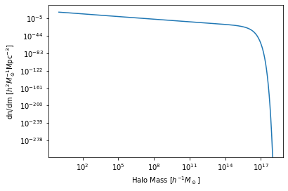
Let’s have a look at the halo mass function:

plt.plot(hm.m, hm.dndm)
plt.xscale("log")
plt.yscale("log")

plt.xlabel(r"Halo Mass [$h^{-1} M_\odot$]")
plt.ylabel(r"dn/dm [$h^2 M_\odot^{-1} {\rm Mpc}^{-3}$]");

Most often, what is desired is the power spectrum (or auto-correlation function) of the galaxies:

plt.plot(hm.k_hm, hm.power_auto_tracer, label="Galaxy-Galaxy Power")
plt.plot(hm.k_hm, hm.power_1h_auto_tracer, ls="--", label="1-halo term")
plt.plot(hm.k_hm, hm.power_2h_auto_tracer, ls="--", label="2-halo term")


plt.xscale("log")
plt.yscale("log")

plt.ylim(1e-5, 1e6)
plt.legend()
plt.xlabel("Wavenumber [h/Mpc]")
plt.ylabel(r"Galaxy Power Spectrum [${\rm Mpc^3} h^{-3}$]");

You can check all the quantities that are available with

hm.quantities_available()

['ERROR_ON_BAD_MDEF',
 '_central_occupation',
 '_corr_mm_base_fnc',
 '_dlnsdlnm',
 '_do_1halo_integral',
 '_find_m_min',
 '_get_corr_2h_auto_fnc',
 '_get_naive_bias_effective',
 '_get_power_2h_auto_fnc',
 '_get_power_2h_primitive',
 '_growth_factor_fn',
 '_gtm',
 '_matter_exclusion',
 '_normalisation',
 '_power0',
 '_power_halo_centres_fnc',
 '_r_table',
 '_sigma_0',
 '_tm',
 '_total_occupation',
 '_tracer_exclusion',
 '_unn_sig8',
 '_unn_sigma0',
 '_unnormalised_lnT',
 '_unnormalised_power',
 'bias',
 'bias_effective_matter',
 'bias_effective_tracer',
 'central_fraction',
 'central_occupation',
 'cmz_relation',
 'colossus_cosmo',
 'corr_1h_auto_matter',
 'corr_1h_auto_matter_fnc',
 'corr_1h_auto_tracer',
 'corr_1h_auto_tracer_fnc',
 'corr_1h_cross_tracer_matter',
 'corr_1h_cross_tracer_matter_fnc',
 'corr_1h_cs_auto_tracer',
 'corr_1h_cs_auto_tracer_fnc',
 'corr_1h_ss_auto_tracer',
 'corr_1h_ss_auto_tracer_fnc',
 'corr_2h_auto_matter',
 'corr_2h_auto_matter_fnc',
 'corr_2h_auto_tracer',
 'corr_2h_auto_tracer_fnc',
 'corr_2h_cross_tracer_matter',
 'corr_2h_cross_tracer_matter_fnc',
 'corr_auto_matter',
 'corr_auto_matter_fnc',
 'corr_auto_tracer',
 'corr_auto_tracer_fnc',
 'corr_cross_tracer_matter',
 'corr_cross_tracer_matter_fnc',
 'corr_halofit_mm',
 'corr_halofit_mm_fnc',
 'corr_linear_mm',
 'corr_linear_mm_fnc',
 'cosmo',
 'delta_k',
 'dndlnm',
 'dndlog10m',
 'dndm',
 'filter',
 'fsigma',
 'growth',
 'growth_factor',
 'halo_bias',
 'halo_concentration',
 'halo_overdensity_crit',
 'halo_overdensity_mean',
 'halo_profile',
 'halo_profile_lam',
 'halo_profile_rho',
 'halo_profile_ukm',
 'hmf',
 'hod',
 'how_big',
 'k',
 'k_hm',
 'linear_power_fnc',
 'lnsigma',
 'm',
 'mass_effective',
 'mass_nonlinear',
 'mdef',
 'mean_density',
 'mean_density0',
 'mean_density_in_halos',
 'mean_tracer_den',
 'mean_tracer_den_unit',
 'n_eff',
 'ngtm',
 'nonlinear_delta_k',
 'nonlinear_power',
 'nonlinear_power_fnc',
 'normalised_filter',
 'nu',
 'power',
 'power_1h_auto_matter',
 'power_1h_auto_matter_fnc',
 'power_1h_auto_tracer',
 'power_1h_auto_tracer_fnc',
 'power_1h_cross_tracer_matter',
 'power_1h_cross_tracer_matter_fnc',
 'power_1h_cs_auto_tracer',
 'power_1h_cs_auto_tracer_fnc',
 'power_1h_ss_auto_tracer',
 'power_1h_ss_auto_tracer_fnc',
 'power_2h_auto_matter',
 'power_2h_auto_matter_fnc',
 'power_2h_auto_tracer',
 'power_2h_auto_tracer_fnc',
 'power_2h_cross_tracer_matter',
 'power_2h_cross_tracer_matter_fnc',
 'power_auto_matter',
 'power_auto_matter_fnc',
 'power_auto_tracer',
 'power_auto_tracer_fnc',
 'power_cross_tracer_matter',
 'power_cross_tracer_matter_fnc',
 'power_hh',
 'r',
 'radii',
 'rho_gtm',
 'rho_ltm',
 'satellite_fraction',
 'satellite_occupation',
 'sd_bias',
 'sd_bias_correction',
 'sigma',
 'total_occupation',
 'tracer_cmz_relation',
 'tracer_concentration',
 'tracer_density_m',
 'tracer_mmin',
 'tracer_profile',
 'tracer_profile_lam',
 'tracer_profile_rho',
 'tracer_profile_ukm',
 'transfer',
 'transfer_function']

Thus we could estimate the total fraction of galaxies in the sample that are satellites:

hm.satellite_fraction

0.4366657267260254

Or get the effective galaxy bias:

hm.bias_effective_tracer

1.0403662203981139

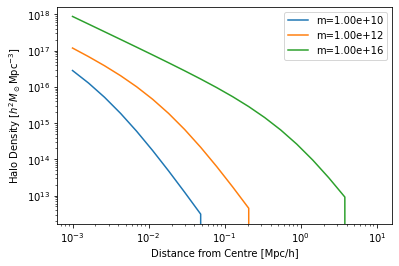
Furthermore, some of the properties of the framework are themselves what we call Components. These are entire objects with their own methods for calculating various quantities (some of which have been exposed to the framework interface if they are commonly used).

For example, the halo_profile object contains methods for evaluating halo-based properties:

r = np.logspace(-3, 1, 20)
for m in [1e10, 1e12, 1e16]:
    plt.plot(r, hm.halo_profile.rho(r=r, m=m), label=f"m={m:1.2e}")

plt.legend()
plt.yscale("log")
plt.xscale("log")

plt.xlabel("Distance from Centre [Mpc/h]")
plt.ylabel(r"Halo Density [$h^2 M_\odot {\rm Mpc}^{-3}$]");

Input Parameters

There are many options for the TracerHaloModel. One of the motivations for halomod is to make it as feature-complete as possible, especially in terms of the input models (and their flexibility).

The documentation for the TracerHaloModel itself does not contain all the possible parameters (as many of them are passed through to super-classes). You can see a full list of available parameters with:

TracerHaloModel.parameter_info()

bias_model : Bias Model.

bias_params : Dictionary of parameters for the Bias model.

cosmo_model : instance of `astropy.cosmology.FLRW` subclass
    The basis for the cosmology -- see astropy documentation. Can be a custom
    subclass. Defaults to Planck18.

cosmo_params : dict
    Parameters for the cosmology that deviate from the base cosmology passed.
    This is useful for repeated updates of a single parameter (leaving others
    the same). Default is the empty dict. The parameters passed must match
    the allowed parameters of `cosmo_model`. For the basic class this is
    :Tcmb0: Temperature of the CMB at z=0
    :Neff: Number of massless neutrino species
    :m_nu: Mass of neutrino species (list)
    :H0: The hubble constant at z=0
    :Om0: The normalised matter density at z=0

n : float
    Spectral index of fluctuations
    Must be greater than -3 and less than 4.

sigma_8 : float
    RMS linear density fluctuations in spheres of radius 8 Mpc/h

growth_params : dict
    Relevant parameters of the :attr:`growth_model`.

lnk_min : float
    Minimum (natural) log wave-number, :attr:`k` [h/Mpc].

lnk_max : float
    Maximum (natural) log wave-number, :attr:`k` [h/Mpc].

dlnk : float
    Step-size of log wave-numbers

z : float
    Redshift.
    Must be greater than 0.

transfer_model : str or :class:`hmf.transfer_models.TransferComponent` subclass, optional
    Defines which transfer function model to use.
    Built-in available models are found in the :mod:`hmf.transfer_models` module.
    Default is CAMB if installed, otherwise EH.

transfer_params : dict
    Relevant parameters of the `transfer_model`.

takahashi : bool
    Whether to use updated HALOFIT coefficients from Takahashi+12.
    If False, use the original coefficients from Smith+2003.

growth_model : `hmf.growth_factor._GrowthFactor` subclass
    The model to use to calculate the growth function/growth rate.

hmf_model : str or `hmf.fitting_functions.FittingFunction` subclass
    A model to use as the fitting function :math:`f(\sigma)`

Mmin : float
    Minimum mass at which to perform analysis [units :math:`\log_{10}M_\odot h^{-1}`].

Mmax : float
    Maximum mass at which to perform analysis [units :math:`\log_{10}M_\odot h^{-1}`].

dlog10m : float
    log10 interval between mass bins

mdef_model : str or :class:`hmf.halos.mass_definitions.MassDefinition` subclass
    A model to use as the mass definition.

mdef_params : dict
    Model parameters for `mdef_model`.

delta_c : float
    The critical overdensity for collapse, :math:`\delta_c`.

hmf_params : dict
    Model parameters for `hmf_model`.

filter_model : :class:`hmf.filters.Filter` subclass
    A model for the window/filter function.

filter_params : dict
    Model parameters for `filter_model`.

disable_mass_conversion : bool
    Disable converting mass function from builtin definition to that provided.

halo_profile_model : The halo density halo_profile model.

halo_profile_params : Dictionary of parameters for the Profile model.

halo_concentration_model : A halo_concentration-mass relation.

halo_concentration_params : Dictionary of parameters for the concentration model.

sd_bias_model : Model of Scale Dependant Bias.

sd_bias_params : Dictionary of parameters for Scale Dependant Bias.

exclusion_model : A string identifier for the type of halo exclusion used (or None).

exclusion_params : Dictionary of parameters for the Exclusion model.

dr_table : The width of r bin.

rmin : Minimum length scale.

rmax : Maximum length scale.

rnum : Number of r bins.

rlog : If True, r bins are logarithmically distributed.

hm_logk_min : The minimum k bin in log10.

hm_logk_max : The maximum k bin in log10.

hm_dlog10k : The width of k bin in log10.

hc_spectrum : The spectrum with which the halo-centre power spectrum is identified.
    Choices are 'linear', 'nonlinear', 'filtered-lin' or 'filtered-nl'.
    'filtered' spectra are filtered with a real-space top-hat window
    function at a scale of 2 Mpc/h, which ensures that haloes
    do not overlap on scales small than this.

force_1halo_turnover : Suppress 1-halo power on scales larger than a few virial radii.

colossus_params : Options for colossus cosmology not set/derived in the astropy cosmology.

hod_params : Dictionary of parameters for the HOD model.

hod_model : :class:`~hod.HOD` class.

tracer_profile_model : The tracer density halo_profile model.

tracer_profile_params : Dictionary of parameters for the tracer Profile model.

tracer_concentration_model : The tracer concentration-mass relation.

tracer_concentration_params : Dictionary of parameters for tracer concentration-mass relation.

tracer_density : Mean density of the tracer, ONLY if passed directly.

Anything listed here can be set at instantiation time. A few common options might be:

hm_smt3 = TracerHaloModel(
    z=3.0,  # Redshift
    hmf_model="SMT",  # Sheth-Tormen mass function
    cosmo_params={"Om0": 0.3, "H0": 70.0},
)

So then we can compare the correlation functions for each of our defined models:

plt.plot(hm.r, hm.corr_auto_tracer, label="Tinker at z=0")
plt.plot(hm_smt3.r, hm_smt3.corr_auto_tracer, label="SMT at z=3")

plt.xscale("log")
plt.yscale("log")

plt.xlabel("r [Mpc/h]")
plt.ylabel("Correlation Function");

---------------------------------------------------------------------------
IndexError                                Traceback (most recent call last)
Cell In[15], line 1
----> 1 plt.plot(hm.r, hm.corr_auto_tracer, label="Tinker at z=0")
      2 plt.plot(hm_smt3.r, hm_smt3.corr_auto_tracer, label="SMT at z=3")
      4 plt.xscale("log")

File ~/work/halos/halomod/src/halomod/halo_model.py:1514, in TracerHaloModel.corr_auto_tracer(self)
   1511 @property
   1512 def corr_auto_tracer(self):
   1513     """The tracer auto correlation function."""
-> 1514     return self.corr_auto_tracer_fnc(self.r)

File ~/work/halos/halomod/src/halomod/halo_model.py:1509, in TracerHaloModel.corr_auto_tracer_fnc.<locals>.<lambda>(r)
   1506 @property
   1507 def corr_auto_tracer_fnc(self):
   1508     """A callable returning the tracer auto correlation function."""
-> 1509     return lambda r: self.corr_1h_auto_tracer_fnc(r) + self.corr_2h_auto_tracer_fnc(r)

File ~/work/halos/halomod/.venv/lib/python3.12/site-packages/hmf/_internals/_cache.py:114, in cached_quantity.<locals>._get_property(self)
    111     activeq.add(name)
    113 # Go ahead and calculate the value -- each parameter accessed will add itself to the index.
--> 114 value = f(self)
    115 setattr(self, prop, value)
    117 # Invert the index

File ~/work/halos/halomod/src/halomod/halo_model.py:1488, in TracerHaloModel.corr_2h_auto_tracer_fnc(self)
   1485 @cached_quantity
   1486 def corr_2h_auto_tracer_fnc(self):
   1487     """A callable returning the 2-halo term of the tracer auto-correlation."""
-> 1488     return self._get_corr_2h_auto_fnc(
   1489         self._tracer_exclusion, self.bias_effective_tracer, debias=False
   1490     )

File ~/work/halos/halomod/src/halomod/halo_model.py:762, in DMHaloModel._get_corr_2h_auto_fnc(self, exclusion, effective_bias, debias)
    758 power_primitive = self._get_power_2h_primitive(exclusion, effective_bias, debias=debias)
    760 # Need to set h smaller here because this might need to be transformed back
    761 # to power.
--> 762 corr = tools.hankel_transform(power_primitive, self._r_table, "r", h=1e-4)
    764 return tools.ExtendedSpline(
    765     self._r_table, corr, lower_func="power_law", upper_func=tools._zero
    766 )

File ~/work/halos/halomod/src/halomod/tools.py:69, in hankel_transform(f, trns_var, trns_var_name, h, chunksize, atol, rtol)
     67 prev_res = 100
     68 res = 0
---> 69 p = f[ir] if hasattr(f, "__len__") else f
     70 while not np.isclose(prev_res, res, atol=atol, rtol=rtol) and nn < nmax:
     71     prev_res = res

IndexError: list index out of range

Notice that the first time we accessed hm.corr_auto_tracer it took a few moments to return, because it was computing. Now, however, it will return instantly:

%timeit hm.corr_auto_tracer

Some of the parameters passed into TracerHaloModel are more complex than simply setting a redshift. Many of the parameters themselves define whole Components. Every one of these has two associated parameters: component_model and component_params. You’ve already seen one of these – the hmf_model. There is an associated hmf_params which sets arbitrary model-specific parameters, and should be passed as a dictionary. In fact, you saw one of those too: cosmo_params.

Once you’ve created the object, the actual model instance is available simply as component (so for example, hm.hmf is a full class instance containing methods for calculating \(f(\sigma)\)).

You can check out what parameters are available for a specific model (and their current values) by printing the .params variable of the Component. For example:

hm_smt3.hmf.params

thus, passing hmf_params = {'A':0.3} would set up a component with different parameters, making it easy to explore parameter space (or constrain those parameters via a fitting/MCMC routine!).

Updating parameters in-place

Once you have a framework created, you can update parameters in-place fully consistently. So, if we wanted to update our halo profile to be a Hernquist model:

hm.halo_profile_model = "Hernquist"

To ensure it has been properly updated, let’s create a new instance:

hm_orig = TracerHaloModel()

And plot the halo profiles:

plt.plot(hm._r_table, hm.halo_profile_rho[:, -1], label="Hernquist")
plt.plot(hm._r_table, hm_orig.halo_profile_rho[:, -1], label="NFW")

plt.xscale("log")
plt.yscale("log")
plt.legend(loc="lower left")
plt.text(3, 1e-2, f"Halo Mass = {hm.m[-1]:1.2e}", fontsize=13)

plt.xlabel("Distance from Centre [Mpc/h]")
plt.ylabel(r"Halo Density [$h^2 M_\odot {\rm Mpc}^{-3}$]");

halomod inherits the caching system of hmf, which means that any updated parameter will automatically invalidate the cache for all dependent quantities, updating them on the next time they are accessed.

Whirlwind Tour of Components and Models

There are many different kinds of Components that offer several different models each. Let’s take a look at some that you could choose from:

• Cosmology: All FLRW cosmologies are supported via astropy.

• Transfer Functions: several commonly-used forms of the transfer function are provided, including: BBKS, BondEfs, CAMB, EH, FromFile.

• Growth Factor: default is to solve the standard integral in a flat-LCDM cosmology, though one can also use the output from CAMB which supports arbitrary non-flat FLRW cosmologies. Several other approximations are also implemented (eg. GenMFGrowth and Carroll1992).

• Filters: filters (or window-functions) are convolved with the density field to define “regions” of space associated with overdensities. The standard filter is the TopHat (in real-space), but you may also choose other filters such as the Gaussian, SharpK or SharpKEllipsoid.

• Mass Definitions: we provide several standard halo mass definitions (i.e. the definition of what makes a halo a halo). These include FoF, SOMean, SOCritical and SOVirial. Explicitly defining the mass definitions allows conversions to be made between definitions.

• Fitting Functions: we provide many mass function fits reported in the literature, including favourites such as SMT, PS, Jenkins01 and Tinker08.

• Halo Bias: Used to bias haloes with respect to the background clustering. Options include standards such as SMT01 and Tinker10. Also provided is a generic interface to use bias functions from the COLOSSUS package.

• Halo Profiles: halomod implements an extensive system of subclasses for halo density profiles. These will compute the density profile itself, the cumulative mass distribution, the virial radius, the normalized fourier transform of the density profile, and its self-convolution. They all have a consistent API. Models include NFW, Moore, Hernquist and Einasto.

• Concentration-Mass Relations: To fully specify a halo profile, one must have a model for the halo concentration. We provide several such models, including Bullock01, Duffy08 and Ludlow16. We again provide an interface to use concentration relations from the COLOSSUS package.

• HOD Models: To link galaxies to the DM haloes, we require a halo occupation distribution. A full-featured system of such models is included, and specific models from certain papers are also included, such as those from Zheng05 and Zehavi05. HOD models are not limited to point-tracers like galaxies – they are generic enough that smooth occupation distributions can be modelled, for example the occupation of neutral hydrogen.

• Halo Exclusion: to increase fidelity of the auto-power spectra on transition scales between the 1- and 2-halo terms, various forms of “halo exclusion” have been proposed. We implement simple models such as Sphere exclusion, as well as more complex schemes such as DblSphere, DblEllipsoid and NgMatched (from Tinker+2005).

The API Documentation has an exhaustive listing of your options for these components and their models. The key point is that halomod is built to be a system in which these various components can be mixed and matched consistently.

Along with these components, there are many ways to use halomod. We’ve seen the TracerHaloModel, but you may also be interested in the ProjectedCF (projected correlation function), which performs integrals over the line-of-sight, or the AngularCF which produces the angular correlation function. Furthermore, a set of extensions to Warm Dark Matter models is also provided.

Defining Your Own Models

We’ve seen that using a new model for a particular Component is as simple as passing its string name. However, you can also pass a class directly. For example, to switch to the Bullock01 concentration-mass relation:

from halomod.concentration import Bullock01

hm.halo_concentration_model = Bullock01
hm.mdef_model = "SOCritical"

plt.plot(hm.m, hm.cmz_relation)
plt.xscale("log")
plt.yscale("log")

plt.xlabel(r"Mass [$M_\odot/h$]")
plt.ylabel("Halo Concentration");

This also lets you easily define your own models. For example, say we had a crazy idea and thought that a constant concentration (with mass) was a good idea. We could create such a model:

from hmf.halos.mass_definitions import SOCritical

from halomod.concentration import CMRelation

class ConstantConcentration(CMRelation):
    native_mdefs = (SOCritical(),)
    _defaults = {"amplitude": 3}

    def cm(self, m, z=0):
        return self.params["amplitude"] * np.ones_like(m)

Notice that we inherited from CMRelation, which provides a basic set of methods that we don’t need to define ourselves, and also provides an interface that we must adhere to. In particular, any parameters that should be changeable by the user should be specified (with defaults) in the _defaults dictionary. Also, a cm method must be implemented which returns the concentration as a function of mass, for a particular redshift. The user-changeable parameters are available as self.params.

We can now instantly use this new definition:

hm.halo_concentration_model = ConstantConcentration

plt.plot(hm.m, hm.cmz_relation)
plt.xscale("log")
plt.yscale("log")

plt.xlabel(r"Mass [$M_\odot/h$]")
plt.ylabel("Halo Concentration");

And we can see what effect this would have on the power spectrum:

plt.plot(hm.k_hm, hm.power_auto_matter, label="Constant Concentration")
plt.plot(hm_orig.k_hm, hm_orig.power_auto_matter, label="Duffy08 Concentration")

plt.xscale("log")
plt.yscale("log")
plt.xlim(3e-3, 100)
plt.ylim(1e-1, 1e5)

plt.legend()
plt.xlabel("Wavenumber [h/Mpc]")
plt.ylabel(r"Galaxy Power Spectrum [${\rm Mpc^3} h^{-3}$]");

Every single Component allows you to create models in this fashion. Some, like the Profile, implement a very rich set of functionality for free (for the halo profile, you need only specify one function – the halo density profile itself – for a full range of functionality to be available).