Cross-Correlations with halomod

The cornerstone of halomod is the TracerHaloModel, which defines the behaviour of dark matter halos and one specific tracer within them. If you want to cross-correlate different tracers, extracting different quantities from two different halo models and calculate the cross-correlation, you can use CrossCorrelations framework. This tutorial goes through a simple example of such a calculation.

import numpy as np
from halomod.cross_correlations import CrossCorrelations,_HODCross, ConstantCorr
import matplotlib.pyplot as plt
import halomod

print(f"Using halomod v{halomod.__version__}")

Using halomod v1.6.1.dev3+ge514be1.d20200819

A CrossCorrelations object essentially needs three inputs: halo models for two different tracers, and a cross_hod_model to specify how these two tracers cross-correlate, which typically should be constructed by users themselves. Let’s first use a very basic ConstantCorr relation (we’ll go back to what it is later):

cross = CrossCorrelations(
    cross_hod_model=ConstantCorr,
    halo_model_1_params={'z': 1},
    halo_model_2_params={'z': 0}
)

This defines the cross-correlation between the same galaxy distribution (the default Zehavi05) at z=1.0 and z=0.0.

The two halo models within the cross-correlation can be easily extracted and manipulated as they are just TracerHaloModel objects. For example, if we want to change the redshift of the cross-correlation:

print(cross.halo_model_1.z)
cross.halo_model_1.z = 0.5
print(cross.halo_model_1.z)

1.0
0.5

The various two-point statistics of this cross-correlation:

plt.plot(cross.halo_model_1.r,cross.corr_cross-1, ls='-', label='total')
plt.plot(cross.halo_model_1.r,cross.corr_2h_cross, ls='--', label='2-halo')
plt.plot(cross.halo_model_1.r,cross.corr_1h_cross, ls=':', label='1-halo')
plt.xscale('log')
plt.yscale('log')
plt.ylim(1e-5,1e5)
plt.legend()
plt.ylabel(r'$\xi_{\rm cross}$')
plt.xlabel(r'r [Mpc/h]');

/home/steven/Documents/Projects/halos/HMF/hmf/src/hmf/density_field/halofit.py:106: UserWarning: sigma_8 is not used any more, and will be removed in v4
  warnings.warn("sigma_8 is not used any more, and will be removed in v4")

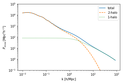
plt.plot(cross.halo_model_1.k_hm,cross.power_cross, ls='-', label='total')
plt.plot(cross.halo_model_1.k_hm,cross.power_2h_cross, ls='--', label='2-halo')
plt.plot(cross.halo_model_1.k_hm,cross.power_1h_cross, ls=':', label='1-halo')
plt.xscale('log')
plt.yscale('log')
plt.ylim(1e-1,1e5)
plt.legend()
plt.ylabel(r'$P_{\rm cross}\,[{\rm Mpc^3 h^{-3}}]$')
plt.xlabel(r'k [h/Mpc]');

The Cross-Correlated HOD

Now let’s get to the difficult part of cross_hod. To understand how to construct it we need to go through the math first. The 2-halo term is easy enough:

\[ \begin{align}\begin{aligned} P_{\rm 2h}^{\rm ij}(k) = b_{\rm i}(k) b_{\rm j}(k) P_m (k),\\where :math:`b_{\rm i,j}` is the effective bias of tracers i,j against the underlying matter power spectrum\end{aligned}\end{align} \]

\[ \begin{align}\begin{aligned} b_{\rm i,j} = \frac{1}{\bar{\rho}_{\rm i,j}} \int {\rm d}m\,n(m)\, b(m)\, \langle T_{\rm i}(m) \rangle\, \tilde{u}_{\rm i}(k|m).\\Here :math:`\rho` is the density of the tracer, :math:`n(m)` is the halo mass function, :math:`b(m)` is the linear halo bias, :math:`\langle T_{\rm i}(m) \rangle` is the total HOD and :math:`\tilde{u}_{\rm i}(k|m)` is the normalized satellite density profile in Fourier space.\end{aligned}\end{align} \]

As shown above, the 2-halo term can be determined entirely by the halo models of the two tracers with no extra information needed. However, it is not the case with 1-halo term:

\[ \begin{align}\begin{aligned}\begin{split} \begin{split} P_{\rm 1h}^{\rm ij}(k) = \frac{1}{\bar{\rho}_{\rm i}\bar{\rho}_{\rm j}}\int {\rm d}m\,n(m) \Big[& \langle T_{\rm i}^{\rm c} T_{\rm j}^{\rm s} \rangle u_{\rm j}(k|m)\\ +&\langle T_{\rm i}^{\rm s} T_{\rm j}^{\rm c} \rangle u_{\rm i}(k|m)\\ +&\langle T_{\rm i}^{\rm s} T_{\rm j}^{\rm s} \rangle u_{\rm i}(k|m)u_{\rm j}(k|m) \Big] \end{split}\end{split}\\where c,s denotes centre and satellite components. The problem here is that we don't know how different :math:`\langle T_{\rm i}^{\rm c,s} T_{\rm j}^{\rm c,s} \rangle` correlates.\end{aligned}\end{align} \]

The way halomod deals with this is to define:

\[\langle T_{\rm i}^{\rm c} T_{\rm j}^{\rm s} \rangle = \langle T_{\rm i}^{\rm c} \rangle \langle T_{\rm j}^{\rm s} \rangle + \sigma_{\rm i}^{\rm c}\sigma_{\rm j}^{\rm s} R_{\rm ij}^{\rm cs}\]

\[\langle T_{\rm i}^{\rm s} T_{\rm j}^{\rm c} \rangle = \langle T_{\rm i}^{\rm s} \rangle \langle T_{\rm j}^{\rm c} \rangle + \sigma_{\rm i}^{\rm s}\sigma_{\rm j}^{\rm c} R_{\rm ij}^{\rm sc}\]

\[ \begin{align}\begin{aligned} \langle T_{\rm i}^{\rm s} T_{\rm j}^{\rm s} \rangle = \langle T_{\rm i}^{\rm s} \rangle \langle T_{\rm j}^{\rm s} \rangle + \sigma_{\rm i}^{\rm s}\sigma_{\rm j}^{\rm s} R_{\rm ij}^{\rm ss} - Q\\where :math:`\sigma^{\rm c,s}` is the standard deviation of HOD, :math:`-1\leq R_{\rm ij} \leq 1` describes the correlation between two probes and :math:`Q` is the expected number of self-pairs at zero separation. These quantities are, to first order, functions of halo mass :math:`m`. Note :math:`R_{\rm ij}^{\rm cs}` and :math:`R_{\rm ij}^{\rm sc}` are two different quantities.\end{aligned}\end{align} \]

With this in mind we can define our cross_hod. Suppose we want to cross-correlate two different galaxy samples that follow different HODs. The base class for all cross-correlation HODs is _HODCross, upon which we construct some model. For simplicity, let us consider the scenario where \(R_{\rm ij}\) are some constants and there are no self-pairs:

class ConstantCorr(_HODCross):
    """Correlation relation for constant cross-correlation pairs"""

    _defaults = {"R_ss": 0.0, "R_cs": 0.0, "R_sc": 0.0}

    def R_ss(self, m):
        return self.params["R_ss"]

    def R_cs(self, m):
        return self.params["R_cs"]

    def R_sc(self, m):
        return self.params["R_sc"]

    def self_pairs(self, m):
        """The expected number of cross-pairs at a separation of zero."""
        return 0

Note this is just an illustration and this class is already included in halomod as we imported it above. Constructing CrossCorrelations:

cross = CrossCorrelations(
    cross_hod_model=ConstantCorr,
    halo_model_1_params=dict(hod_model = 'Zehavi05'),
    halo_model_2_params=dict(hod_model = 'Zheng05')
)

We can update the parameters \(R_{\rm ij}\):

# Setting all of the R parameters to one is saying that the two samples
# are completely correlated -- i.e. the same sample. This will give back
# an autocorrelation.
cross.cross_hod_params = dict(R_ss = 1.0,R_sc = 1.0,R_cs = 1.0)
power_1_tot = cross.power_cross
power_1_2h = cross.power_2h_cross
power_1_1h = cross.power_1h_cross

# On the other end of the scale, setting all to zero means the two
# samples are entirely independent. This of course will almost never
# be completely true, since most samples are at least causally connected
# to the underlying halo.
cross.cross_hod_params = dict(R_ss = 0.0,R_sc = 0.0,R_cs = 0.0)
power_2_tot = cross.power_cross
power_2_2h = cross.power_2h_cross
power_2_1h = cross.power_1h_cross

plt.plot(cross.halo_model_1.k_hm,power_1_tot, ls='-', label='total R=1')
plt.plot(cross.halo_model_1.k_hm,power_1_2h, ls='--', label='2-halo R=1')
plt.plot(cross.halo_model_1.k_hm,power_1_1h, ls=':', label='1-halo R=1')
plt.plot(cross.halo_model_1.k_hm,power_2_tot, ls='-', label='total R=0')
plt.plot(cross.halo_model_1.k_hm,power_2_2h, ls='--', label='2-halo R=0')
plt.plot(cross.halo_model_1.k_hm,power_2_1h, ls=':', label='1-halo R=0')
plt.xscale('log')
plt.yscale('log')
plt.ylim(1e-1,1e5)
plt.legend()
plt.ylabel(r'$P_{\rm cross}\,[{\rm Mpc^3 h^{-3}}]$')
plt.xlabel(r'k [h/Mpc]');

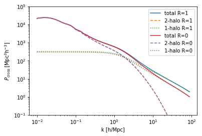
As one can see, the 2-halo terms are the same whereas the 1-halo term varies with the choice of R.

When trying to construct a realistic cross-correlation, you may need to find some empirical description of R as functions of halo mass. Furthermore, note that the HODs used above are Poisson, and therefore have well-defined \(\sigma\) that can be calculated from centre and satellite hod. If you use customized HOD models, make sure you define the sigma_satellite and sigma_central attributes (on the HOD model, not the _HODCross model).