A Showcase of Components in halomod

In this demo, we will showcase each and every one of the different models and components in halomod, to give a taste of its capabilities. Note that the plots generated in this notebook appear in THIS PAPER.

import halomod
import hmf
import numpy as np
print(f"Using halomod v{halomod.__version__}")
print(f"Using hmf v{hmf.__version__}")
from halomod.bias import make_colossus_bias
from halomod.concentration import make_colossus_cm

Using halomod v1.6.1.dev3+ge514be1.d20200819
Using hmf v3.3.4.dev14+g9a9b63c.d20210610

Setup Matplotlib

%matplotlib inline

import matplotlib.pyplot as plt

from matplotlib import rc, rcParams

Since these plots will be included in a paper, we define some preset configurations for different kinds of plots, to achieve some consistency.

paper_font_size = 10  # elsarticle

def single_column(height_ratio=1/1.5):
    linewidth = 3.49  # Get this in your tex using \printinunitsof{in}\prntlen{\linewidth}
    paper_settings(linewidth, height_ratio)


def two_column(height_ratio = 1/1.5):
    textwidth = 7.22  # Get this in your tex using \printinunitsof{in}\prntlen{\textwidth}
    paper_settings(textwidth, height_ratio)

def paper_settings(width, height_ratio = 1/1.5):
    plt.style.use("seaborn-paper")

    rc('figure', figsize=(width, width * height_ratio), dpi=200)
    rc(('xtick', 'ytick'), labelsize=paper_font_size - 2, direction='in')
    rc('legend', fontsize=paper_font_size-1, frameon=False, columnspacing=1, handletextpad=0.4)
    rc('axes', labelsize=paper_font_size-1)

    rc("savefig", dpi=600, bbox='tight')

Setup default model

Some of the components presented here can be calculated using lower-level frameworks, but all of them can be calculated from the TracerHaloModel, so we use this.

from halomod import TracerHaloModel

base_model = TracerHaloModel(
    dr_table = 0.03,
    dlnk = 0.05,
    dlog10m = 0.05,
    transfer_params={
        'kmax':1e2
    }
)

# Pre-compute many of the relevant quantities
base_model.power_auto_tracer;

recalcing dndm

/home/steven/Documents/Projects/halos/HALOMOD/halomod/src/halomod/halo_model.py:1250: RuntimeWarning: overflow encountered in double_scalars
  c[i] = tools.spline_integral(self.m, intg, xmin=10 ** mmin)
/home/steven/Documents/Projects/halos/HMF/hmf/src/hmf/density_field/halofit.py:106: UserWarning: sigma_8 is not used any more, and will be removed in v4
  warnings.warn("sigma_8 is not used any more, and will be removed in v4")

Since most of the plots we make will be comparing all possible models of a particular component, we define a simple function to find all the models for a particular component:

import importlib

def get_models(module, base_class, ignore=()):
    mod = importlib.import_module(module)
    cls = getattr(mod, base_class)

    out = []
    for v in mod.__dict__.values():
        try:
            if issubclass(v, cls) and v != cls and v.__name__ not in ignore:
                out.append(v)
        except TypeError:
            pass
    return out

For bias models:

get_models('halomod.bias', 'Bias')

[halomod.bias.UnityBias,
 halomod.bias.Mo96,
 halomod.bias.Jing98,
 halomod.bias.ST99,
 halomod.bias.SMT01,
 halomod.bias.Seljak04,
 halomod.bias.Seljak04Cosmo,
 halomod.bias.Tinker05,
 halomod.bias.Mandelbaum05,
 halomod.bias.Pillepich10,
 halomod.bias.Manera10,
 halomod.bias.Tinker10,
 halomod.bias.Tinker10PBSplit]

Now, define a function that will do most of the plotting for us. It will grab all the models defined for a particular component, and plot a resulting quantity for all of them, with a lower panel showing the ratio to the fiducial model.

import random

def model_comparison_plot(
    module, component, attr_name, x, y, ignore=(),
    height_ratio=1/1.5, ylab=None, y_unit = None,
    yratio_lab = None, ylog=True, comparison_limits=(0.8, 1.2), xlim=None,
    ylim=None, must_include=(),
    ncol_legend=1, legend_size=None, max_models=10, extra_models=None,
    extra_params=None
):
    extra_params=extra_params or {}
    extra_models = extra_models or []
    # Get all the models for this component
    models = get_models(module, component, ignore)
    if extra_models:
        models += extra_models

    # Limit them to seven models (randomly)
    if len(models) > max_models:
        print(f"Randomly choosing {max_models} out of {len(models)} models.")
        tmp_models = [m for m in models if m.__name__ in must_include or m in extra_models]
        for m in tmp_models:
            models.remove(m)

        models = random.sample(models, max_models - len(tmp_models))
        models.extend(tmp_models)

    # Most model comparison plots will be single column in the paper.
    single_column(height_ratio)

    subplot_kw = {"xscale": 'log'}
    if xlim:
        subplot_kw['xlim'] = xlim

    # Create a two-panel plot with the lower panel slightly smaller.
    fig, ax = plt.subplots(
        2, 1, sharex=True,
        gridspec_kw={"hspace": 0, 'height_ratios': [3, 2]},
        subplot_kw=subplot_kw
    )

    # Plot the different models.
    model = base_model.clone()  # Make a new updateable model.
    for i, cmp_model in enumerate(models):
        if cmp_model.__name__ != getattr(base_model, attr_name).__name__:
            model.update(**{attr_name.replace("model", 'params'): extra_params.get(cmp_model.__name__, {})})

        model.update(**{attr_name: cmp_model})
        if cmp_model in extra_models:
            ls = ':'
        else:
            ls = ['-', '--', ':'][i//10]

        xx = getattr(model, x)
        if x == 'nu':
            xx = np.sqrt(xx)
        ax[0].plot(xx, getattr(model, y), label=cmp_model.__name__, lw=1, ls=ls)
        ax[1].plot(xx, getattr(model, y) / getattr(base_model, y), ls=ls)

    if ylog:
        ax[0].set_yscale('log')

    ax[0].legend(ncol=ncol_legend, fontsize=legend_size or rcParams['legend.fontsize'])

    ylab = ylab or y

    # Set axis labels and limits.
    if y_unit:
        ylabel = f"{ylab} [{y_unit}]"
    else:
        ylabel = ylab

    ax[0].set_ylabel(ylabel)
    if x == 'k':
        ax[1].set_xlabel("k [$h$ / Mpc]")
    elif x == 'm':
        ax[1].set_xlabel("m [$h^{-1} M_\odot$]")
    elif x == 'nu':
        ax[1].set_xlabel(r"Peak-height, $\nu$")

    if yratio_lab is None:
        yratio_lab = ylab

    ax[1].set_ylabel(r"%s / $%s_{\rm %s}$" %(yratio_lab, yratio_lab.replace("$", ""), getattr(base_model, attr_name).__name__))
    ax[1].set_ylim(comparison_limits)

    if ylim:
        ax[0].set_ylim(ylim)

    # Save the figure
    plt.savefig(f"plots/{attr_name}s.pdf")

Transfer Function

First, transfer functions. We omit the models that require user input (eg. FromFile).

The transfer function determines the linear power spectrum, which in turn affects the halo mass function (more power on larger scales means more high-mass halos).

model_comparison_plot(
    module="hmf.density_field.transfer_models",
    component = 'TransferComponent',
    ignore=('FromFile','FromArray', 'EH'),
    attr_name = 'transfer_model',
    x = 'k',
    y = 'power',
    ylab = r"$P_{\rm lin}(k)$",
    y_unit = r"$h^{-3}{\rm Mpc}^3$",
    xlim = (1e-4, 1e2),
    yratio_lab = r"$P^{\rm lin}$",
    height_ratio = 1/1.2,
    ncol_legend=2,
    ylim=(1e-4, 1e5),
    comparison_limits=(0.8, 1.25)
)
plt.savefig("/home/steven/Desktop/transfer_models.pdf")

SOMean(200) {'overdensity': 200}
SOMean(200) {'overdensity': 200}
SOMean(200) {'overdensity': 200}
SOMean(200) {'overdensity': 200}
SOMean(200) {'overdensity': 200}

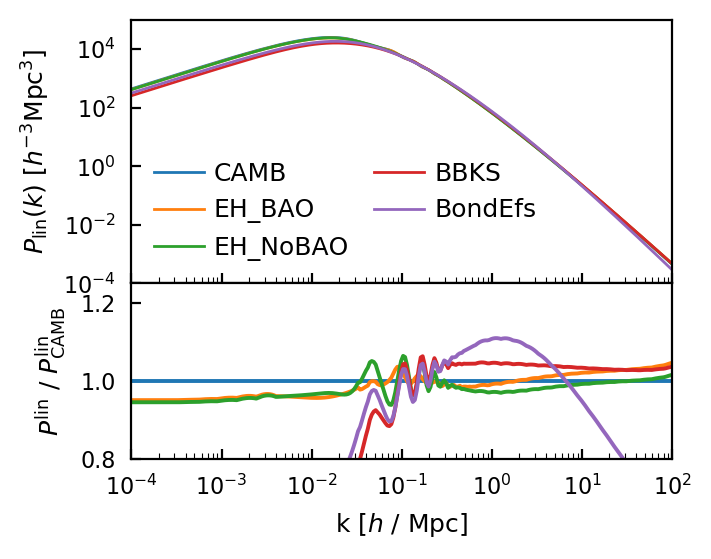
First notice that the fiducial model is CAMB (this is only true if camb is installed, otherwise it is EH_BAO). Since CAMB has BAOs, all the models without BAOs show up in the ratio as having wiggles. Interestingly, CAMB has much higher power on small scales than the other models. CAMB is much slower to run than the other analytic models.

The normalization difference on large scales is due to the difference in the integral of the power spectrum, which is normalized to be the same value via \(\sigma_8\).

Mass Definitions

Here we plot the change in mass and concentration when moving from one mass definition to another.

from hmf.halos.mass_definitions import SOMean, SOCritical, SOVirial, FOF

single_column(height_ratio=1/1.5)


fig, ax = plt.subplots(
    2, 1, sharex=True,
    gridspec_kw={"hspace": 0, 'height_ratios': [3, 2]},
    subplot_kw={"xscale": 'log'}
)

for mdef in [SOMean(overdensity=300), SOCritical(overdensity=300), SOVirial(), FOF()]:
    m, r, c = base_model.mdef.change_definition(
        base_model.m,
        mdef=mdef,
        profile=base_model.halo_profile,
        cosmo=base_model.cosmo
    )

    ax[0].plot(base_model.m, m / base_model.m, label=mdef.colossus_name)
    ax[1].plot(base_model.m, c / base_model.cmz_relation)

ax[0].grid(True)
ax[1].grid(True)

ax[0].legend(ncol=2, frameon=True)

ax[0].set_ylabel(r"$m_{\rm new} / m_{\rm old}$")
ax[1].set_ylabel(r"$c_{\rm new} / c_{\rm old}$")
ax[1].set_xlabel("m, [$h^{-1}M_{\odot}$]")

plt.savefig("plots/mass_conversion.pdf")

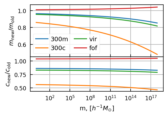
Notice that halos with a higher overdensity threshold move to lower masses and lower concentration.

Window Functions / Filters

The filter model, \(W(x)\), is convolved with the power spectrum to produce the mass variance (which in turn is used to define the halo mass function). Optimally, the shape of the filter model is matched to the shape of primordial patches that become halos. However, typically a simplified model such as a top-hat is used.

model_comparison_plot(
    module="hmf.density_field.filters",
    component = 'Filter',
    attr_name = 'filter_model',
    x = 'm',
    y = 'sigma',
    ylab = r"$\sigma(m)$",
    yratio_lab = r"$\sigma$",
    height_ratio = 1/1.2,
    ncol_legend=1,
    ylim=(0, 10),
    ylog=False,
    xlim=(1e8, 1e16),
    comparison_limits = (0.7, 1.3)
)

(100000000.0, 1e+16)

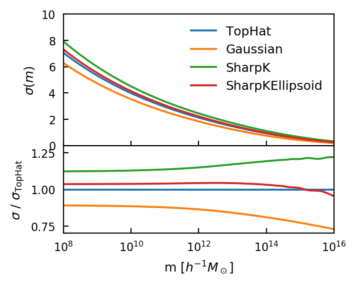
Note that while any of these can be used to generate \(\sigma(m)\), the normalisation of the power spectrum, \(\sigma(R=8)\), is always calculated using the TopHat.

Mass Function

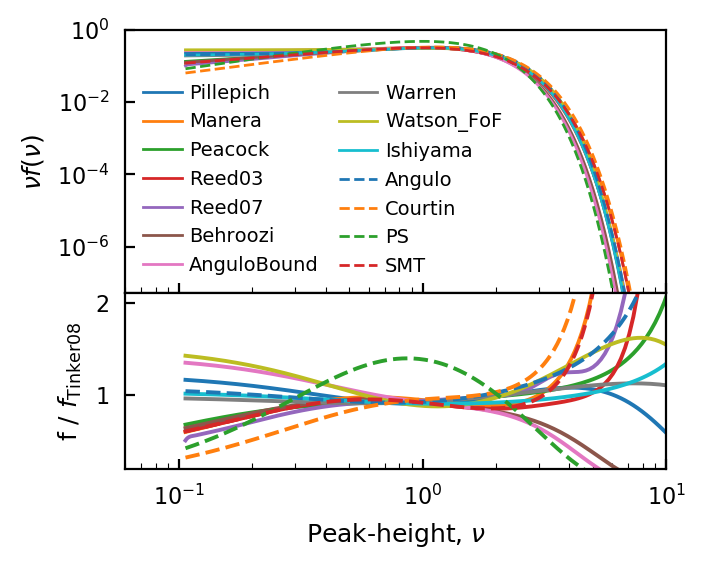
There are many fitting functions for the HMF included in hmf. Some are fitted against FOF-haloes, while others are fitted to SO halos of various definitions. Here we’ll only plot a few, so that the plot is not too confusing.

model_comparison_plot(
    module="hmf.mass_function.fitting_functions",
    component = 'FittingFunction',
    attr_name = 'hmf_model',
    x = 'nu',
    y = 'fsigma',
    ylab = r"$\nu f(\nu)$",
    height_ratio = 1/1.2,
    ncol_legend=2,
    ylim=(5e-8, 1),
    #ylog=False,
    xlim=(6e-2, 1e1),
    comparison_limits = (0.2, 2.1),
    must_include = ("PS", "SMT"),
    ignore=("ST", "Jenkins"),  # Jenkins gets in the way of the legend
    legend_size=7,
    max_models = 14,
    yratio_lab = "f"
)
plt.savefig("/home/steven/Desktop/hmf_models.pdf")

Randomly choosing 14 out of 19 models.

/home/steven/Documents/Projects/halos/HALOMOD/halomod/src/halomod/concentration.py:132: UserWarning: Requested mass definition 'FoF(l=0.2)' is not in native definitions for the 'Duffy08' CMRelation. No mass conversion will be performed, so results will be wrong. Using 'FoF(l=0.2)'.
  f"Requested mass definition '{mdef}' is not in native definitions for "

Bias

The halo bias describes the clustering strength of halos of a given mass compared to the background matter. Many bias models are included in halomod, but even more can be accessed through the interface to colossus:

comparat = make_colossus_bias("comparat17")
bhat11 = make_colossus_bias("bhattacharya11")

model_comparison_plot(
    module="halomod.bias",
    component = 'Bias',
    attr_name = 'bias_model',
    x = 'nu',
    y = 'halo_bias',
    ylab = r"b($\nu$)",
    height_ratio = 1/1.2,
    ncol_legend=2,
    comparison_limits = (0.5, 1.6),
    must_include = ('Tinker05', 'Mandelbaum05', "ST99", "SMT01", 'Mo96', 'Jing98'),
    ignore=("UnityBias", "Seljak04Cosmo"),
    legend_size = 7,
    max_models=11,
    xlim=(6e-2, 1e1),
    ylim=(3e-1, 2e3),
    extra_models=[
        comparat,
        bhat11
    ]
)

Randomly choosing 11 out of 13 models.
WARNING: Astropy cosmology class contains massive neutrinos, which are not taken into account in Colossus.
WARNING: Astropy cosmology class contains massive neutrinos, which are not taken into account in Colossus.

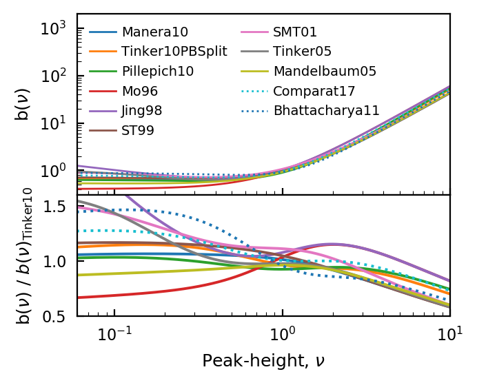
Concentration

The concentration-mass relation affects the shape of the halo profile at different masses. halomod includes physically-motivated forms (eg. Bullock and Ludlow) and power-law forms. Since the power-law forms are really only applicable to a single cosmology, we focus on the analytic forms in this plot:

model_comparison_plot(
    module="halomod.concentration",
    component = 'CMRelation',
    attr_name = 'halo_concentration_model',
    x = 'm',
    y = 'cmz_relation',
    ylab = r"c(m)",
    yratio_lab = "c",
    height_ratio = 1/1.2,
    ncol_legend=2,
    comparison_limits = (0.3, 2.1),
    ignore=("Ludlow2016", "Ludlow2016Empirical", "Zehavi11", "Bullock01Power"),
    legend_size = 7,
    ylim=(2, 3e2),
    xlim=(7e7, 5e15),
    extra_models = [
        make_colossus_cm('prada12'),
        make_colossus_cm('diemer15'),
        make_colossus_cm('diemer19'),
#        make_colossus_cm('ishiyama20'),
    ]
)

/home/steven/Documents/Projects/halos/HALOMOD/halomod/src/halomod/concentration.py:130: UserWarning: Requested mass definition 'SOMean(200)' is not in native definitions for the 'Bullock01' CMRelation. No mass conversion will be performed, so results will be wrong. Using 'SOMean(200)'.
  f"Requested mass definition '{mdef}' is not in native definitions for "
/home/steven/Documents/Projects/halos/HALOMOD/halomod/src/halomod/concentration.py:130: UserWarning: Requested mass definition 'SOMean(200)' is not in native definitions for the 'Ludlow16' CMRelation. No mass conversion will be performed, so results will be wrong. Using 'SOMean(200)'.
  f"Requested mass definition '{mdef}' is not in native definitions for "
/home/steven/Documents/Projects/halos/HALOMOD/halomod/src/halomod/concentration.py:130: UserWarning: Requested mass definition 'SOMean(200)' is not in native definitions for the 'Ludlow16Empirical' CMRelation. No mass conversion will be performed, so results will be wrong. Using 'SOMean(200)'.
  f"Requested mass definition '{mdef}' is not in native definitions for "
/home/steven/Documents/Projects/halos/HALOMOD/halomod/src/halomod/concentration.py:538: UserWarning: Only use Ludlow16Empirical c(m,z) relation when using Planck-like cosmology
  "Only use Ludlow16Empirical c(m,z) relation when using Planck-like cosmology"
/home/steven/Documents/Projects/halos/HALOMOD/halomod/src/halomod/concentration.py:130: UserWarning: Requested mass definition 'SOMean(200)' is not in native definitions for the 'Prada12' CMRelation. No mass conversion will be performed, so results will be wrong. Using 'SOMean(200)'.
  f"Requested mass definition '{mdef}' is not in native definitions for "

WARNING: Astropy cosmology class contains massive neutrinos, which are not taken into account in Colossus.

/home/steven/miniconda3/envs/halomod/lib/python3.7/site-packages/colossus/halo/concentration.py:421: UserWarning: Could not find concentration for model prada12, mass 1.12e+17, mdef 200m.
  warnings.warn(msg)
/home/steven/miniconda3/envs/halomod/lib/python3.7/site-packages/colossus/halo/concentration.py:421: UserWarning: Could not find concentration for model prada12, mass 1.26e+17, mdef 200m.
  warnings.warn(msg)
/home/steven/miniconda3/envs/halomod/lib/python3.7/site-packages/colossus/halo/concentration.py:421: UserWarning: Could not find concentration for model prada12, mass 1.41e+17, mdef 200m.
  warnings.warn(msg)
/home/steven/miniconda3/envs/halomod/lib/python3.7/site-packages/colossus/halo/concentration.py:421: UserWarning: Could not find concentration for model prada12, mass 1.58e+17, mdef 200m.
  warnings.warn(msg)
/home/steven/miniconda3/envs/halomod/lib/python3.7/site-packages/colossus/halo/concentration.py:421: UserWarning: Could not find concentration for model prada12, mass 1.78e+17, mdef 200m.
  warnings.warn(msg)
/home/steven/miniconda3/envs/halomod/lib/python3.7/site-packages/colossus/halo/concentration.py:421: UserWarning: Could not find concentration for model prada12, mass 2.00e+17, mdef 200m.
  warnings.warn(msg)
/home/steven/miniconda3/envs/halomod/lib/python3.7/site-packages/colossus/halo/concentration.py:421: UserWarning: Could not find concentration for model prada12, mass 2.24e+17, mdef 200m.
  warnings.warn(msg)
/home/steven/miniconda3/envs/halomod/lib/python3.7/site-packages/colossus/halo/concentration.py:421: UserWarning: Could not find concentration for model prada12, mass 2.51e+17, mdef 200m.
  warnings.warn(msg)
/home/steven/miniconda3/envs/halomod/lib/python3.7/site-packages/colossus/halo/concentration.py:421: UserWarning: Could not find concentration for model prada12, mass 2.82e+17, mdef 200m.
  warnings.warn(msg)
/home/steven/miniconda3/envs/halomod/lib/python3.7/site-packages/colossus/halo/concentration.py:421: UserWarning: Could not find concentration for model prada12, mass 3.16e+17, mdef 200m.
  warnings.warn(msg)
/home/steven/miniconda3/envs/halomod/lib/python3.7/site-packages/colossus/halo/concentration.py:421: UserWarning: Could not find concentration for model prada12, mass 3.55e+17, mdef 200m.
  warnings.warn(msg)
/home/steven/miniconda3/envs/halomod/lib/python3.7/site-packages/colossus/halo/concentration.py:421: UserWarning: Could not find concentration for model prada12, mass 3.98e+17, mdef 200m.
  warnings.warn(msg)
/home/steven/miniconda3/envs/halomod/lib/python3.7/site-packages/colossus/halo/concentration.py:421: UserWarning: Could not find concentration for model prada12, mass 4.47e+17, mdef 200m.
  warnings.warn(msg)
/home/steven/miniconda3/envs/halomod/lib/python3.7/site-packages/colossus/halo/concentration.py:421: UserWarning: Could not find concentration for model prada12, mass 5.01e+17, mdef 200m.
  warnings.warn(msg)
/home/steven/miniconda3/envs/halomod/lib/python3.7/site-packages/colossus/halo/concentration.py:421: UserWarning: Could not find concentration for model prada12, mass 5.62e+17, mdef 200m.
  warnings.warn(msg)
/home/steven/miniconda3/envs/halomod/lib/python3.7/site-packages/colossus/halo/concentration.py:421: UserWarning: Could not find concentration for model prada12, mass 6.31e+17, mdef 200m.
  warnings.warn(msg)
/home/steven/miniconda3/envs/halomod/lib/python3.7/site-packages/colossus/halo/concentration.py:421: UserWarning: Could not find concentration for model prada12, mass 7.08e+17, mdef 200m.
  warnings.warn(msg)
/home/steven/miniconda3/envs/halomod/lib/python3.7/site-packages/colossus/halo/concentration.py:421: UserWarning: Could not find concentration for model prada12, mass 7.94e+17, mdef 200m.
  warnings.warn(msg)
/home/steven/miniconda3/envs/halomod/lib/python3.7/site-packages/colossus/halo/concentration.py:421: UserWarning: Could not find concentration for model prada12, mass 8.91e+17, mdef 200m.
  warnings.warn(msg)
/home/steven/Documents/Projects/halos/HALOMOD/halomod/src/halomod/concentration.py:130: UserWarning: Requested mass definition 'SOMean(200)' is not in native definitions for the 'Diemer15' CMRelation. No mass conversion will be performed, so results will be wrong. Using 'SOMean(200)'.
  f"Requested mass definition '{mdef}' is not in native definitions for "

WARNING: Astropy cosmology class contains massive neutrinos, which are not taken into account in Colossus.

/home/steven/Documents/Projects/halos/HALOMOD/halomod/src/halomod/concentration.py:130: UserWarning: Requested mass definition 'SOMean(200)' is not in native definitions for the 'Diemer19' CMRelation. No mass conversion will be performed, so results will be wrong. Using 'SOMean(200)'.
  f"Requested mass definition '{mdef}' is not in native definitions for "

WARNING: Astropy cosmology class contains massive neutrinos, which are not taken into account in Colossus.

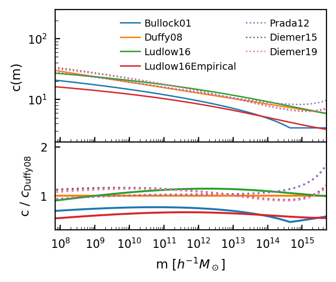
Notice that both of the physical forms have discontinuities, which arise when the predicted redshift of formation for a given halo mass is less than zero. This typically does not present a problem for the halo model, for which intermediate masses are the most important.

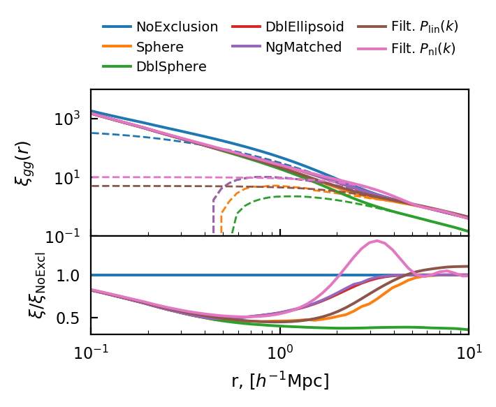
Halo Exclusion

model = base_model.clone()

single_column(height_ratio=1/1.5)

fig, ax = plt.subplots(
    2, 1, sharex=True,
    gridspec_kw={"hspace": 0, 'height_ratios': [3, 2]},
    subplot_kw={"xscale": 'log'}
)

for i, excl in enumerate(['NoExclusion', 'Sphere', 'DblSphere_', 'DblEllipsoid_', 'NgMatched_']):
    model.exclusion_model = excl

    ax[0].plot(model.r, model.corr_auto_tracer, label=excl.replace("_", ""), color=f'C{i}')
    ax[0].plot(model.r, model.corr_2h_auto_tracer, ls='--', color=f'C{i}', lw=1)
    ax[1].plot(model.r, model.corr_auto_tracer / base_model.corr_auto_tracer)

model.exclusion_model = 'NoExclusion'

model.hc_spectrum = 'filtered-lin'
ax[0].plot(model.r, model.corr_auto_tracer, label=r"Filt. $P_{\rm lin}(k)$", color=f'C{i+1}')
ax[0].plot(model.r, model.corr_2h_auto_tracer, ls='--', color=f'C{i+1}', lw=1)
ax[1].plot(model.r, model.corr_auto_tracer / base_model.corr_auto_tracer, )

model.hc_spectrum = 'filtered-nl'
ax[0].plot(model.r, model.corr_auto_tracer, label=r"Filt. $P_{\rm nl}(k)$", color=f'C{i+2}')
ax[0].plot(model.r, model.corr_2h_auto_tracer, ls='--', color=f'C{i+2}', lw=1)
ax[1].plot(model.r, model.corr_auto_tracer / base_model.corr_auto_tracer, )

ax[0].legend(ncol=3, frameon=False, fontsize=7, bbox_to_anchor=(0., 1.02, 1., .102))
ax[0].set_yscale('log')

ax[0].set_xlim(1e-1, 1e1)
ax[0].set_ylim(1e-1, 1e4)
ax[1].set_ylabel(r"$\xi / \xi_{\rm No Excl}$")
ax[0].set_ylabel(r"$\xi_{gg}(r)$")
ax[1].set_xlabel("r, [$h^{-1}$Mpc]")

plt.savefig("plots/halo_exclusion.pdf")

HOD

For the HOD, we’ll only be showing models of point-source-like tracers (i.e. galaxies). A whole set of HOD models for continuous tracers (eg. HI gas) are also available. Also note that these models look very similar to each other. This is by design. Most of the models are essentially nested (i.e. you can get back Zehavi05 from setting some of the Contreras13 parameters to zero or one). By default, halomod sets the parameters so that the model returns the same or a similar occupation function. However, the HOD is not fundamental in nature – it depends on the actual galaxy sample being observed (and its depth/wavelength etc), so these models can vary widely for different parameters.

single_column(height_ratio=1/1.5)

model = base_model.clone()
for hod in ['Zehavi05', 'Zheng05', 'Tinker05',  'Geach12', 'Contreras13']:
    model.hod_model = hod
    plt.plot(model.m, model.total_occupation, label=hod)

plt.xscale('log')
plt.yscale('log')
plt.ylim(1e-4, 1e4)
plt.xlim(1e9, 1e16)
plt.legend(fontsize=8)

plt.xlabel("m, [$h^{-1}M_\odot$]")
plt.ylabel("N(m)")
plt.savefig("plots/hod_models.pdf")

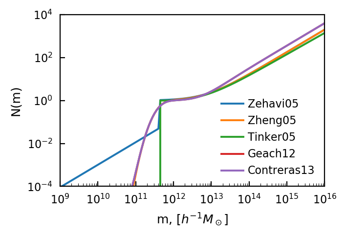
The key things to recognize are a low-mass cutoff, essentially corresponding to the depth of the survey, and a high-mass powerlaw with slope close to one (i.e. doubling halo mass doubles the occupancy). The differentiation between central and satellite halos causes the bump seen above at \(m\sim10^{12}\).

Profiles

two_column(height_ratio=1/2.3)

fig, ax = plt.subplots(
    2, 2, sharex='col',
    gridspec_kw={"hspace": 0, 'height_ratios': [3, 2]},
    subplot_kw={"xscale": 'log'}
)

profiles = get_models("halomod.profiles", 'Profile', ignore=("ProfileInf", "Constant", "NFWInf", "HernquistInf", "MooreInf", "GeneralizedNFWInf"))

model = base_model.clone()
for profile in profiles:
    model.halo_profile_model = profile
    model.halo_profile_params = {'alpha': 1.5} if profile.__name__ == "GeneralizedNFW" else {}
    ax[0, 0].plot(model.r, model.halo_profile.rho(model.r, np.array([1e12])), label=profile.__name__)
    ax[1, 0].plot(model.r, model.halo_profile.rho(model.r, np.array([1e12])) /base_model.halo_profile.rho(model.r, np.array([1e12])))

    ax[0, 1].plot(model.m, model.halo_profile.rho(0.03, model.m), label=profile.__name__)
    ax[1, 1].plot(model.m, model.halo_profile.rho(0.03, model.m) / base_model.halo_profile.rho(0.03, model.m))

ax[0, 0].set_yscale('log')
ax[0, 1].set_yscale('log')

ax[0, 0].set_ylim(1e9, 1e17)
ax[0, 0].set_xlim(1e-2, 0.3)
ax[0, 0].legend(ncol=2, fontsize=8)
ax[1, 0].set_ylim(0.1, 2)

ax[0, 1].set_yscale('log')
#ax[0].set_ylim(1e9, 1e17)
ax[0, 1].set_xlim(1e9, 1e17)

ax[1, 0].set_xlabel(r"r, [$h^{-1}{\rm Mpc}$]")
ax[0, 0].set_ylabel(r"$\rho(r|m)$");

ax[0,0].set_title("m = $10^{12} h^{-1}M_\odot$")
ax[0,1].set_title("r = $0.03 h^{-1}$Mpc")

ax[1, 1].set_xlabel(r"m, [$h^{-1}M_\odot$]")
ax[1, 0].set_ylabel(r"$\rho/\rho_{\rm NFW}$")

plt.savefig("plots/profile_models.pdf")

/home/steven/miniconda3/envs/halomod/lib/python3.7/site-packages/ipykernel_launcher.py:16: RuntimeWarning: invalid value encountered in true_divide
  app.launch_new_instance()
/home/steven/miniconda3/envs/halomod/lib/python3.7/site-packages/ipykernel_launcher.py:19: RuntimeWarning: invalid value encountered in true_divide
/home/steven/miniconda3/envs/halomod/lib/python3.7/site-packages/ipykernel_launcher.py:16: RuntimeWarning: divide by zero encountered in true_divide
  app.launch_new_instance()
/home/steven/miniconda3/envs/halomod/lib/python3.7/site-packages/ipykernel_launcher.py:19: RuntimeWarning: divide by zero encountered in true_divide

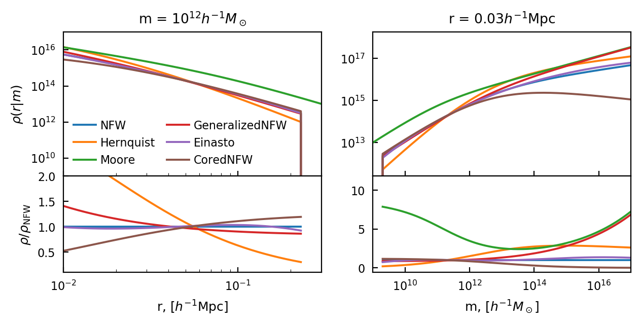
We show here the profile for six models, plotted against mass and radius. We omit the “Inf” versions of each profile, since they are the same but extend to infinity (and are less useful for the halo model itself since some of them contain infinite mass).